Are you still doing some data processing in Excel? Why not try to create an Excel dynamic dashboard to make it clear?
What is Dashboard Chart?
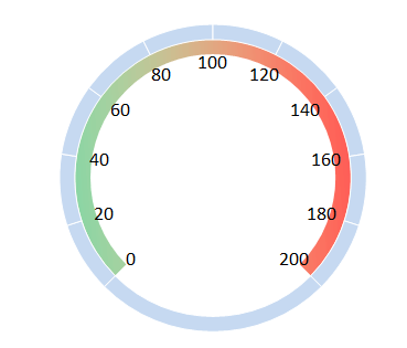
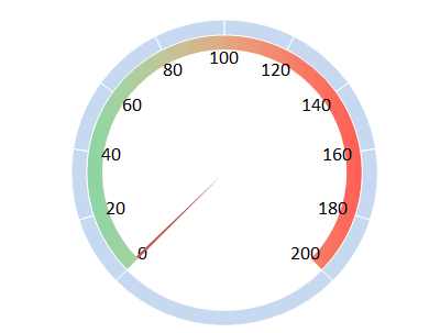
Dashboard chart imitates the speed of car, it can be used to reflect ratio index such as growth rate of income. It’s not only intuitive but also simple for everyone to understand.
Steps to create a Dynamic Dashboard in Excel 2010
There are four components of Dashboard: scale rage, outer circle, inner circle, and warning ribbon. Before you are going to create a dashboard in Excel 2010, you have to download and install XY Chart Labels.
Excel Dashboard Creation Step 1: Create a Doughnut
1: Getting the data as the following picture in Excel 2010. 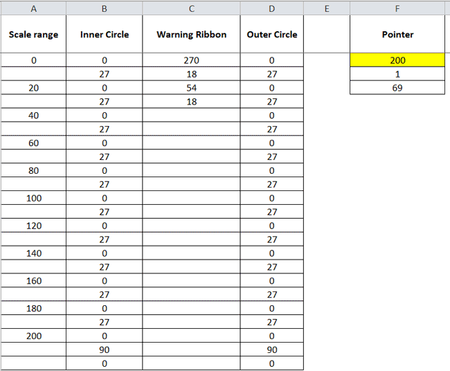
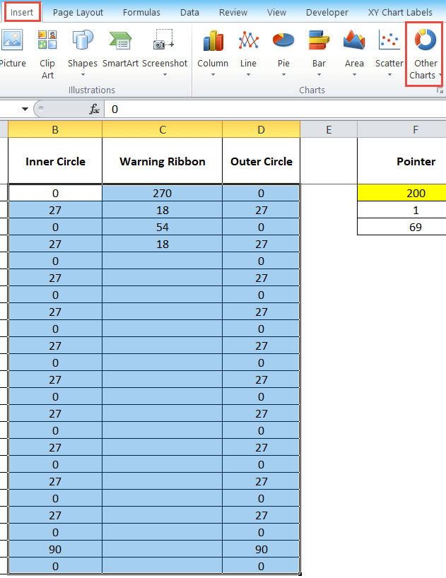
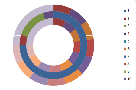
2: Select column B, C, and D. Then expand the OtherCharts under Insert tab and click on Doughnut.
Excel Dashboard Creation Step 2: Change the Doughnut settings
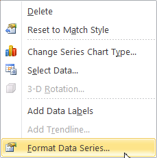
1: Delete the chart legend then right-click on the outer circle and select Format Data Series.
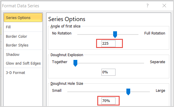
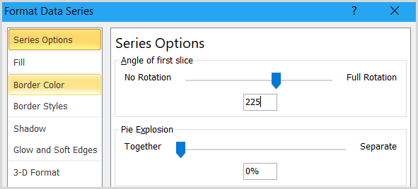
2: Under Series Options section, set the angle of the first slice to 225 degrees and 70% of doughnut hole size.
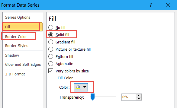
3: In the Fill tab, select a light color to fill the outer circle. Then click on Border Color in the left sidebar, select white.
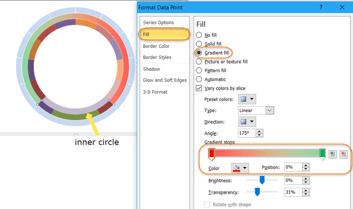
4: Double-click the 270 degrees block of the inner circle then set gradient fill for it. The rest parts fill with white.
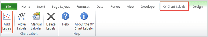
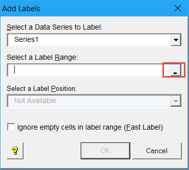
5: Click on warning ribbon and navigate to XY Chart labels > Add labels.
6: Under Select a Label Range, choose A2 – A24 data. Right-click on warning ribbon and fill it with no color.
Excel Dashboard Creation Step 3: Making a Dashboard pointer
1: Choose data below Pointer and make it into a pie chart. Set background color to transparency and remove its legend.

2: Double-click on the chart and input 225 as the angle of first slice. Set the two blocks of 200 degrees and 69 degrees in no color.

3: Adjust the pointer to the right position.
Excel Dashboard Creation Step 4: Make it a Dynamic Dashboard
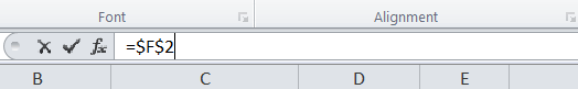
1: Insert a text box at the bottom of dashboard. Select the text box and locate to formula bar. Hit “=” key and click on F2 cell then press Enter.
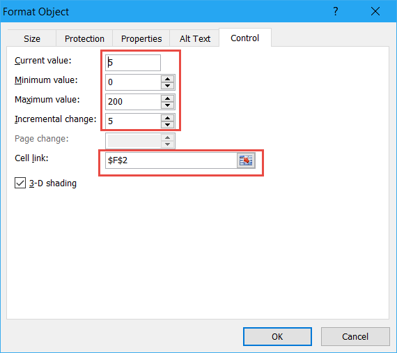
2: Navigate to Developer > Insert, and select a form control.

3: Right-click on the control and select Format Control. In the Control tab, the settings of control are shown below.